A sample of toy FDM code
Solving equation


Time integration is full implicit, and during each time step Newton’s method is employed.
PROGRAM MAIN
!--------------------------------------------------
!Implicit time evolution of equation
!u_t-u''=f(x,u)
!f(x,u)=-2+r*(sin(u)-sin(x^2)),r=2
!--------------------------------------------------
! t=time points
! dt=time step
! h=neighboring nodes distance
! u=unknown
! x=node location
! n=No. of unknowns

!USE SUNPERF

IMPLICIT NONE
INTEGER(4) :: n
REAL(4) :: elapse,time(2),etime
REAL(8) :: t=0,dt=0.1
REAL(8) :: h
REAL(8),ALLOCATABLE :: u(:),x(:)
INTEGER(4) :: count,i

n=50
h=1/(DBLE(n)+1.)
ALLOCATE (x(n),u(n))
x=(/(i*h,i=1,n)/)
u=(/((i*h)**0.5,i=1,n)/)

OPEN(UNIT=100,FILE='data',STATUS='UNKNOWN',ACTION='&
     &WRITE')
DO i=1,n
   WRITE(100,*) t,x(i),u(i)
END DO

DO WHILE (t<1.0)
CALL newton(n,h,dt,u,x)
t=t+dt
DO i=1,n
WRITE(100,*) t,x(i),u(i)
END DO END DO CLOSE(UNIT=100)
elapse=etime(time)
WRITE(*,*) 'elapsed:',elapse
END PROGRAM MAIN
!--------------------------------------------------
SUBROUTINE newton(n,h,dt,u,x)
IMPLICIT NONE
INTEGER(4),INTENT(IN) :: n
REAL(8),INTENT(IN) :: x(n),h,dt
REAL(8),INTENT(INOUT) :: u(n)
REAL(8) :: r=2,c(n),error,b(n,1),b0(n,1),a(2,n)
REAL(8) :: alpha=1.0,beta=-1.0
INTEGER(4) :: info,i,iter
c=u*h*h/dt
iter=0
error=1
DO WHILE (error>1.e-13)
     iter=iter+1
     a(1,:)=-1
     a(2,:)=2+h*h/dt
     b(:,1)=(-2+r*(SIN(u)-SIN(x*x)))*h*h+c
     b(n,1)=b(n,1)+1
     CALL DSBMV('u',n,1,alpha,a,2,u,1,beta,b,1)
     b=-b
     a(2,:)=a(2,:)-r*COS(u)*h*h
     CALL DGTSV(n,1,a(1,2:),a(2,:),a(1,2:),b,n,info)
     error=MAXVAL(ABS(b))
     u=u+b(:,1)
  END DO
  WRITE(*,*) 'INFO',info,'Number of iterations:',iter
END SUBROUTINE newton
!--------------------------------------------------
Output would be like:
% f95 -dalign implicit_newton.f95 -xlic_lib=sunperf
% a.out
 INFO 0 Number of iterations: 4
 INFO 0 Number of iterations: 4
 INFO 0 Number of iterations: 4
 INFO 0 Number of iterations: 4
 INFO 0 Number of iterations: 4
 INFO 0 Number of iterations: 3
 INFO 0 Number of iterations: 3
 INFO 0 Number of iterations: 3
 INFO 0 Number of iterations: 3
 INFO 0 Number of iterations: 3
 elapsed: 0.061407
Of course the exact solution is 


 . Remembering that

 at time
  , then use the BC equations to update the boundary condition. One should remember, the LHS of BC equations use material particle as variable, i.e. in Lagrangian representation. Denote particle on the free surface by
  , MEL is characterized by two steps:
 ;
;


 , elliptic equation for
  and algebra/finite difference for
  . This means for this particular time updating plan, a single linear elliptic equation solver can be used. Remember, this virtue is due to two things, the first is the MEL to eliminate the annoying nonlinear convection term, second, the time splitting using
  (MEL-in mixed-Eulerian-Lagrangian form) or
  (Eulerian form)
 , both the displacement and velocity are functions of time:
 are known as
  . For velocity we have the general time integration:

 means take the derivative within the spatial configuration of time
  . This spatial domain is obtained using velocity updating:
 varies between 0 and 1. When
  , RHS is based on time
 all together, by coupling equation above with mass conservation equation of Eulerian form
  . The other one is try to update velocity separately, for this purpose we have to transform the mass equation, because it is this equation that couples velocities in different directions. On the other hand, we also want to decouple the pressure and velocity. Before introduce the scheme, let’s first take a look at the physical interpretation of the coordnate system.
 , the material particle indexed by
  . In other words, when we talk about some specific material particle, it can be labeled with location
  simply means the
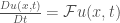
  . By this notation, the momentum equation, assuming constant density and body force, is

![\frac{u_i^{n+1}(x^{n+1})-u^{\ast}(x)}{\Delta t}+\frac{u^{\ast}(x)-u_i^n(x)}{\Delta t}=[-\frac{1}{\rho}\frac{\partial (p^{n+1}-p^n)}{\partial x_i}]+[-\frac{1}{\rho}\frac{\partial p^n}{\partial x_i}+\mu\frac{1}{\rho}\frac{\partial^2 u_i^{\ast}}{\partial x_j\partial x_j}+f_i]](https://s0.wp.com/latex.php?latex=%5Cfrac%7Bu_i%5E%7Bn%2B1%7D%28x%5E%7Bn%2B1%7D%29-u%5E%7B%5Cast%7D%28x%29%7D%7B%5CDelta+t%7D%2B%5Cfrac%7Bu%5E%7B%5Cast%7D%28x%29-u_i%5En%28x%29%7D%7B%5CDelta+t%7D%3D%5B-%5Cfrac%7B1%7D%7B%5Crho%7D%5Cfrac%7B%5Cpartial+%28p%5E%7Bn%2B1%7D-p%5En%29%7D%7B%5Cpartial+x_i%7D%5D%2B%5B-%5Cfrac%7B1%7D%7B%5Crho%7D%5Cfrac%7B%5Cpartial+p%5En%7D%7B%5Cpartial+x_i%7D%2B%5Cmu%5Cfrac%7B1%7D%7B%5Crho%7D%5Cfrac%7B%5Cpartial%5E2+u_i%5E%7B%5Cast%7D%7D%7B%5Cpartial+x_j%5Cpartial+x_j%7D%2Bf_i%5D&bg=fff&fg=444444&s=0&c=20201002)

 :
:
 sequentially. This means to solve two spatial domain PDEs for the first two equations, and take one derivative for the last.
 , spatial problem is (to skip the boundary condition)
 and
and  are global operators in the spatial domain. At each time like
  is resolved and used to update the spatial configuration using
 or
or  ? And to the next step, when one tries to solve (this is so called “time integration”, because it’s discrete version of taking integral) differential equation of